Showing posts with label g09. Show all posts

03 August 2016

630. Making MO figures in gabedit using fchk files from gaussian on Windows XP

The goal is to show how to make pretty figures of MOs from Gaussian computations using GabEdit.

This is a write-up for a colleague whom is using Windows. The GabEdit bits work pretty much the same way on linux, although the povray stuff is a lot easier (in my opinion anyway) on that OS.

Anyway, Windows it is.


A. Optional: Install Gaussian (G09W)
If you have G09W you can install it. To use the formchk utility, add the location of your gaussian installation to path.

Do this by right-clicking on My Computer, select the Advanced tab, click on Environment Variables, and then click on the Path entry under System Variables. Click Edit, and add
;c:\g09w
if that's the correct path for you. The ";" is just to separate your entry from the previous one. If you need to add another entry afterwards (e.g. for povray), put a ";" after c:\g09w


Either way it's optional, as you will likely have access to formchk on the same computer/system that you ran your job on and can do the chk -> fchk conversion there.

Also, using formchk on a windows computer on a .chk file from a linux computer might not work (which was my case)

An alternative is to set up a smallish linux VM: https://verahill.blogspot.com.au/2016/08/631-small-linux-installation-in.html


B. Optional: Add option to open terminal using mouse
Following this: https://stackoverflow.com/questions/378319/windows-explorer-command-prompt-here/379804

Create a plain text file called context.reg


Edit it and put the following in it:

Windows Registry Editor Version 5.00
[HKEY_LOCAL_MACHINE\SOFTWARE\Classes\Folder\shell\cmd]
@="Open Command Prompt Here"
[HKEY_LOCAL_MACHINE\SOFTWARE\Classes\Folder\shell\cmd\command]@="cmd.exe /k pushd %L"

Like so...
Run it (i.e. double-click):
Yes!
You will now have an "Open Command Prompt Here" option when right-clicking on a folder in the file explorer.
Open terminal here
Why do this? Because it makes it easier to run either formchk or povray in the directory where you have your files.


C. Install gabedit
Got to https://sites.google.com/site/allouchear/Home/gabedit/download and get "The Gabedit installer for Windows (OpenGL)"

Run. It's that easy.

When running gabedit for the first time you may be asked lots of questions. You can probably just accept all the defaults. We'll change some of them below.

D. Install povray
Download http://www.povray.org/redirect/www.povray.org/ftp/pub/povray/Official/povwin-3.7-agpl3-setup.exe and also accept to install the editor dlls at the end of the installation.
Download povray
Once that's done, add povray to path. Go to My Computer, right-click, click on the Advanced tab, select Environment Variables, click on path under System Variables and then Edit. Add
;C:\Program Files\POV-Ray\v3.7\bin

Like So


Let's get going!

1. Optional: Convert chk to fchk using formchk
Didn't work for me, but you can always try (I convert the files under linux)

Either way, you must have the fchk file before going to gabedit


2. Open fchk file in gabedit
You need to do a bit of setting up:

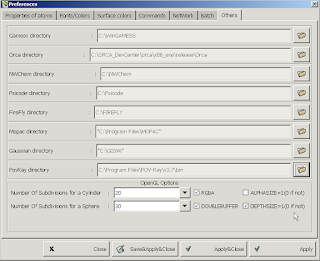
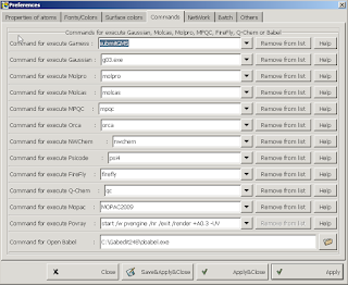
Set path and command for povray


To look at the fchk file:
a) Go to Display
Display Geometry/Orbitals/Density/Vibration


b) unset dipole (because otherwise you'll have an annoying arrow in your figure)
Untick dipole

c) Set desired atom colours.
In particular, I change N from dark blue to light blue so that it doesn't interfere with the orbital colours.
Atom colour

d) Set backgrounds (povray and screen) to white
Povray background

Window background


e) load fchk file
Go to Orbitals/Gaussian fchk


Open your fchk file


f) Set ball/stick parameters
Set Ball and Stick parameters
Apply

g) select level/MO
Note that you get the alpha OR beta orbitals. For a spin restricted system these are the same (apart from signage)

You should edit number of points. 65 is the default. 80 is slow but manageable. 90 is pushing it. Higher = smoother.

Computing...

"Get Isovalue" almost never works properly. Try 0.04-0.06.

Et voilá!
To select a different MO, go back to orbitals and click on Selection.
Selection

h) Edit surfaces
You can change colours and transparency
Transparency is an option

Adjust the transparency/opacity here
i) Export pov
To make a publication-worthy figure, export as pov
Export as Povray
Clicking 'Run' occasionally leads to crash, so it's safer to click on save. Make sure that the background in white.

Edit the command to +A0.01 instead of +A0.3 for less 'pixelated' figure on zooming in. Takes a bit longer to render though. The H/W values depend on your window shape.

Select save, not Run


3. Render povray
You now have a pov file (example.pov). The most straight-forward way to render it is to open the command prompt (terminal) in the same folder and run
pvengine +A0.01 +H604 +W620 example.pov
Rendering

assuming that the H/W values are the ones listed (or multiples of them) when you saved the pov file (it'll be listed in example.bat in the same folder).

And it looks like this:
A basic POV-Ray generated png


You can also run the .bat file associated with the pov file, but note that you'll have to put paths in "":
You need ""s
You can also render in the povray editor (open the povray with the editor):
Povray editor


Render Settings

The issue becomes the default H/W (resolution) values. Override using command line options: +HXXX +WYYY
You may have to associate .pov files with pvengine manually:

Edit -- but you'll be told that there's no program


Select a program to open


pvengine


Always use the selected program

18 January 2016

626. Briefly: Gaussian and cloud computing -- Gaussian G09D with Slurm on aws/ec2

Note: you may want to install awscli and euca2ools. I didn't, so I don't actually know whether they are useful.

My instructions are quite rudimentary since I don't have much time to write these blog posts anymore. Hopefully there's enough information to get you through.


AWS
Either way, sign up for AWS. If you already have an amazon ID I think you can use that. Go to https://aws.amazon.com/

Select Launch an Instance and pick the ubuntu AIM and do Launch and Review. I launched it as a t2.micro instance type, as it is free and it's sufficient for set up but not to run jobs.

Hit launch, and create a new key pair. I called mine myfirstkeypair and saved the pem file in my ~/Downloads folder

In my Downloads folder:
ssh -i "myfirstkeypair.pem" ubuntu@ec2-11-222-33-444.us-west-2.compute.amazonaws.com
I then set a password in the ubuntu AWS image:
sudo passwd ubuntu

I added my id_rsa.pub to ~/.ssh/authorized_keys on the ubuntu AWS image to make logging in via ssh easier -- that way I won't need the pem file.


Set up Gaussian
I then connected with SCP and uploaded my gaussian files -- I went straight for EM64T G09D. It went quite fast at +5 MB/s

scp E6L-103X.tgz ubuntu@ec2-00-111-22-333.us-west-2.compute.amazonaws.com:/home/ubuntu/E6L-103X.tgz

Once that was done, on the ubuntu AWS instance I did:
sudo apt-get install csh 
sudo mkdir /opt/gaussian
cd /opt 
sudo chown ubuntu gaussian -R
cd /opt/gaussian
cp ~/E6L-103X.tgz .
tar xvf E6L-103X.tgz
cd g09
csh bsd/install

echo 'export GAUSS_EXEDIR=/opt/gaussian/g09/bsd:/opt/gaussian/g09/local:/opt/gaussian/g09/extras:/opt/gaussian/g09' >> ~/.bashrc
echo 'export GAUSS_SCRDIR=/home/ubuntu/scratch' >> ~/.bashrc
echo 'export PATH=$PATH:/opt/gaussian/g09' >> ~/.bashrc
source ~/.bashrc 
mkdir ~/scratch ~/jobs

NOTE that you can't run any gaussian jobs under a t2.micro instance. You will have to stop and relaunch as at least a t2.small instance or the jobs will be 'Killed' (that's what is echoed in the terminal when you try to run)
Note that if you terminate an image it will be deleted.

Stop the image and then create a snapshot or an image from it to keep everything you've installed.

Set up Slurm
You'll want a queue manager so that you can launch several jobs in serial. Also, you can set up your script so that it shuts down the image when your job is done to save money.

sudo apt-get update
sudo apt-get install slurm-llnl

ControlMachine=localhost ControlAddr=127.0.0.1 MpiDefault=none ProctrackType=proctrack/pgid ReturnToService=2 SlurmctldPidFile=/var/run/slurm-llnl/slurmctld.pid SlurmdPidFile=/var/run/slurm-llnl/slurmd.pid SlurmdSpoolDir=/var/lib/slurm-llnl/slurmd SlurmUser=slurm StateSaveLocation=/var/lib/slurm-llnl/slurmctld SwitchType=switch/none TaskPlugin=task/none FastSchedule=1 SchedulerType=sched/backfill SelectType=select/linear AccountingStorageType=accounting_storage/none ClusterName=rupert JobAcctGatherType=jobacct_gather/none SlurmctldLogFile=/var/log/slurm-llnl/slurmctld.log SlurmdLogFile=/var/log/slurm-llnl/slurmd.log NodeName=localhost NodeAddr=127.0.0.1 PartitionName=All Nodes=localhost
sudo /usr/sbin/create-munge-key
Edit /etc/default/munge:
OPTIONS=--force
Then run
sudo service slurm-llnl restart
sudo service munge restart 
Test using slurm.batch
#!/bin/bash # #SBATCH -p All #SBATCH --job-name=test #SBATCH --output=res.txt # #SBATCH --ntasks=1 #SBATCH --time=10:00 srun hostname srun sleep 60
and submit with
sbatch slurm.batch
 squeue
             JOBID PARTITION     NAME     USER ST       TIME  NODES NODELIST(REASON)
                 2       All     test   ubuntu  R       0:08      1 localhost

Benchmark:
#!/bin/csh #SBATCH -p All #SBATCH --time=9999999 #SBATCH --output=slurm.out #SBATCH --job-name=benchmark setenv GAUSS_SCRDIR /home/ubuntu/scratch setenv GAUSS_EXEDIR /opt/gaussian/g09/bsd:/opt/gaussian/g09/local:/opt/gaussian/g09/extras:/opt/gaussian/g09 /opt/gaussian/g09/g09< benchmark.in > benchmark.out
Using the same opt/freq benchmark as in post 621.

c4.2xlarge 2h 11 min [1h 20 min] 8 vcpu/16 Gb
c4.4xlarge 1h 15 min [     44 min] 16 vcpu/32 Gb
c4.8xlarge      41 min [     25 min] 36 vcpu/60 Gb

It scales surprisingly well, although not perfectly linearly. It's clear that it's cheaper to use a smaller instance, so if time isn't critical or the larger memory isn't needed, c4.8xlarge is not the first choice.

Dropbox:
You might want to use dropbox to transfer files back and forth, especially finished job files (useful if you shut down the machine using a slurm script as shown below)

cd ~ && wget -O - "https://www.dropbox.com/download?plat=lnx.x86_64" | tar xzf -
~/.dropbox-dist/dropboxd
This computer isn't linked to any Dropbox account... Please visit https://www.dropbox.com/cli_link_nonce?nonce=0011223344556677889900aabbccddeef to link this device. This computer isn't linked to any Dropbox account...

Open that link in a browser, then go back to the terminal.
 
wget -O - https://www.dropbox.com/download?dl=packages/dropbox.py > dropbox.py
sudo mv dropbox.py /usr/local/bin
sudo chmod +x d/usr/local/bin/dropbox.py
dropbox.py autostart y

Now, since you don't want to use up space unnecessarily (you're paying for it after all), exclude as many directories as possible. To exclude all existing dropbox dirs, do
 
cd ~/Dropbox
dropbox.py exclude add `ld -d */`
dropbox.py exclude add `ld *.*`
dropbox.py exclude list

Note that it can't handle directories with spaces in the name, so you'll need to polish the list by hand. Next create a directory where you want to run and store your jobs,e .g.
mkdir ~/Dropbox/aws_jobs

When you run a gaussian job, make sure to specify where the .chk files should end up, e.g.
%chk=/home/ubuntu/scratch/benchmark.chk
so that you don't use up space/bandwidth for your chk files (unless of course you want to).

Stop after execution:
Use a batch script along these lines:
#!/bin/csh #SBATCH -p All #SBATCH --time=9999999 #SBATCH --output=slurm.out #SBATCH --job-name=benchmark setenv GAUSS_SCRDIR /home/ubuntu/scratch setenv GAUSS_EXEDIR /opt/gaussian/g09/bsd:/opt/gaussian/g09/local:/opt/gaussian/g09/extras:/opt/gaussian/g09 /opt/gaussian/g09/g09< benchmark.in > benchmark.out rm /home/ubuntu/scratch/*.* sudo shutdown -h now

28 August 2015

623. Comparing frequency calculations in G09 and NWChem -- the importance of grid density

The vibrational entropy term will differ between calculations done in gaussian and nwchem unless you use "grid xfine" in nwchem. That the grid density is important is nothing new, but the magnitude of the effect on the entropy surprised me.

The difference can be large -- 30 cal/molK for [PPh4]+ at pbe0/cc-pvdz -- which becomes quite significant when multiplied by T (e.g. 298.15 K).

Note that the rotational entropy term also may differ, but that this would be due to different uses of symmetry in the calculations: http://molecularmodelingbasics.blogspot.com.au/2012/12/conformational-and-rotational-entropy.html

If you turn off symmetry (noautosym) in nwchem the rotational entropy will not be corrected. I've noticed that Gaussian, on the other hand, will sneakily apply correction if it finds an acceptable symmetry even if you request nosymm, so make sure that you scan through the output carefully.

Either way, vibrational entropy is not symmetry dependent. Instead you will have to worry about the grid fine-ness when comparing outputs.

If your molecule is very small, such as benzene or tetramethylphosphonium, it seems that you don't have to worry about this. However, even fairly small molecules such as [PPh4]+ will be affected.

Conv. Dens. = Convergence Density


CodeSymmGridConv. Dens.DFT EnergyZPEHCorrS(tot)S(trans)S(rot)S(vib)
G09NF1E-8-1266.584241520.3705160.389751147.07643.35835.00968.708
G09NU1E-8-1266.584303740.3704640.389691146.82943.35835.00968.461
NWNX1E-8-1266.584552230.3703480.389549146.69743.33934.99468.365
NWNX1E-5-1266.584552220.3703480.389549146.70443.33934.99468.371
NWYF1E-5-1266.584536840.3700340.385683118.02343.33933.61741.067
NWYF1E-8-1266.584536840.3700340.385683118.02343.33933.61741.067
NWNF1E-5-1266.584549280.3700340.385683119.39443.33934.99441.062
NWNF1E-8-1266.584549290.3700340.385683119.39443.33934.99441.061
NWYX1E-5-1266.584552740.3703480.389549145.33143.33933.61768.376
NWYX1E-8-1266.584552750.3703480.389549145.33743.33933.61768.382

F=fine. X=Extrafine. U=Ultrafine.
S(rot) values in blue are symmetry corrected. That's completely normal.

With "grid fine" NWChem gives a very different result to G09.

You can see the difference in the predicted IR spectra as well.

Fine (NWChem) (blue rings) vs G09 (red circles):
"grid xfine" (NWChem) (blue rings) vs G09 (red circles):


04 June 2015

610. Opening G09 output files in ECCE. A rough method

Update: Note that one thing that's not recognised at the moment are the MOs. Somehow I don't think that should be too difficult. Likewise, I think one should be able to import nwchem files by a little bit of editing like below.

Original post:
When opening a gaussian output file with the ECCE viewer:
* a symlink to the file is put in a subdirectory of /tmp
* the file is parsed for indications as to what the file type is:
+go+cd /tmp/ecce_me/jobs/Gaussian03__HEa24c +go+ln -s /home/me/calcs/test/Outputs/g03.g03out g03.g03out; echo CMDSTAT=$status CMDSTAT=0 +go+grep "Gaussian 98, Revision" g03.g03out; echo CMDSTAT=$status CMDSTAT=1 +go+grep "Gaussian 94, Revision" g03.g03out; echo CMDSTAT=$status CMDSTAT=1 +go+grep "Gaussian 03, Revision" g03.g03out; echo CMDSTAT=$status CMDSTAT=1 +go+grep "%begin%input" g03.g03out; echo CMDSTAT=$status CMDSTAT=1 +go+grep "%begin%input" g03.g03out; echo CMDSTAT=$status CMDSTAT=1 +go+grep "Northwest Computational Chemistry Package" /home/me/test/Outputs/g03.g03out; echo CMDSTAT=$status
That's easy enough to fool by simply putting a Gaussian 03 line in the output (assuming that the G09 and G03 output are similar enough).

Here's a successful example, in the sense that ECCE found that it was a Gaussian 03 file:
CMDSTAT=0 +go+grep "Gaussian 98, Revision" g03.g03out; echo CMDSTAT=$status CMDSTAT=1 +go+grep "Gaussian 94, Revision" g03.g03out; echo CMDSTAT=$status CMDSTAT=1 +go+grep "Gaussian 03, Revision" g03.g03out; echo CMDSTAT=$status Gaussian 03, Revision CMDSTAT=0 +go+if (-w /tmp/ecce_me/jobs/Gaussian03__7491Sb) echo TRUE TRUE +go+echo $PATH; echo CMDSTAT=$status Word too long. +go+if (-x Gaussian-03.expt) echo TRUE +go+exit; echo GOODBYE exit; echo GOODBYE

However, it fails to detect that Gaussian-03.expt is present and executable (both of which are true).

[SOLUTION]

To sort that out and to enable G09 detection, edit apps/data/client/cap/Gaussian-03.edml:
465 <output mimetype="chemical/x-gaussian03-output" type="parse" verifypattern="Gaussian 09, Revision">g03.g03out</output> 466 <output mimetype="chemical/x-gaussian-03-output" type="parse" verifypattern="Gaussian 09, Revision">g03.out</output> 467 <output mimetype="chemical/x-gaussian03-output" type="parse" verifypattern="Gaussian 03, Revision">g03.g03out</output> 468 <output mimetype="chemical/x-gaussian-03-output" type="parse" verifypattern="Gaussian 03, Revision">g03.out</output> .. 480 <importer>${ECCE_HOME}/scripts/parsers/Gaussian-03.expt </importer>
Your G09 files should now open properly (most of the time).

My ecce_env is fine and my runtime_setup.sh file is called by bash, but somehow it wouldn't find the Gaussian-03.expt file. Maybe it has something to do with the use of csh -f

NOTE that the file isn't imported -- it's just opened. It would've been nice if you could actually import the calculation into ECCE. Still, being able to view it is a nice start. 

09 April 2014

570. Briefly: restarting a g09 frequency job with SGE, using same queue

I've had g09 frequency jobs die on me, and in g09 analytical frequency jobs can only be restarted using the .rwf. Because the .rwf files are 160 gb, I don't want to be copying them back and forth between nodes. It's easier then to simply make sure that the restarted job is run on the same node as the original job.

A good resource for SGE related stuff is http://rous.mit.edu/index.php/SGE_Instructions_and_Tips#Submitting_jobs_to_specific_queues

Either way, first figure out what node the job ran on. Assuming that the job number was 445:
qacct -j 445|grep hostname
hostname compute-0-6.local

Next figure out the PID, as this is used to name the Gau-[PID].rwf file:
grep PID g03.g03out
Entering Link 1 = /share/apps/gaussian/g09/l1.exe PID= 24286.

You can now craft your restart file, g09_freq.restart -- you'll need to make sure that the paths are appropriate for your system:
%nprocshared=8 %Mem=900000000 %rwf=/scratch/Gau-24286.rwf %Chk=/home/me/jobs/testing/delta_631gplusstar-freq/delta_631gplusstar-freq.chk #P restart
(having empty lines at the end of the file is important) and a qsub file, g09_freq.qsub:
#$ -S /bin/sh #$ -cwd #$ -l h_rt=999:30:00 #$ -l h_vmem=8G #$ -j y #$ -pe orte 8 export GAUSS_SCRDIR=/tmp export GAUSS_EXEDIR=/share/apps/gaussian/g09/bsd:/share/apps/gaussian/g09/local:/share/apps/gaussian/g09/extras:/share/apps/gaussian/g09 /share/apps/gaussian/g09/g09 g09_freq.restart > g09_freq.out
Then submit it to the correct queue by doing
qsub -q all.q@compute-0-6.local g09_freq.qsub

The output goes to g09_freq.log. You know if the restart worked properly if it says
Skip MakeAB in pass 1 during restart.
and
Resume CPHF with iteration 214.

Note that restarting analytical frequency jobs in g09 can be a hit and miss affair. Jobs that run out of time are easy to restart, and some jobs that die silently have also been restarted successfully. On the other hand, a job that died because my resource allocations ran out couldn't be restarted i.e. restart started the freq job from scratch. The same happened with one a node of mine that has what seems like a dodgy PSU. Finally, I also couldn't restart jobs that died silently due to allocation all the RAM to g09 without leaving any to the OS (or at least that's the current best theory). It may thus be a good idea to back up the rwf file every now and again, in spite of the unwieldy size.

05 February 2014

550. Briefly: Getting ECCE to work with Gaussian 09 (G09) part 2: Geometry trace when using NoSymm

I've made a couple of posts about how to modify ECCE to work better in general, but in particular with Gaussian 09  (G09).

See here for some of the previous posts:
Adding new basis sets, part 1: http://verahill.blogspot.com.au/2013/06/455-adding-nwchem-basis-sets-to-ecce.html
Adding new basis sets, part 2:  http://verahill.blogspot.com.au/2013/06/456-adding-nwchem-basis-sets-to-ecce.html
Adding new exchange/correlation functionals:
http://verahill.blogspot.com.au/2013/12/533-adding-new-exchangecorrelation.html
Adding new options to ECCE
http://verahill.blogspot.com.au/2013/12/534-adding-new-options-to-ecce-adding.html
Getting ECCE to read frequency calc output from G09 calcs:
http://verahill.blogspot.com.au/2013/12/536-briefly-getting-ecce-to-work-with.html


Either way, I've noticed that when I'm using the NoSymm option during optimisation ECCE fails to import the geometries from the geometry steps.
No geometry trace option


What is even worse is that if you use an optimisation job like that as the basis for another job by selecting Duplicate Setup with Last Geometry ECCE will in fact use the starting geometry -- not the optimised one.

Luckily the fix is simple -- edit apps/parsers/gaussian-03.desc and add the following lines:
[GEOMTRACE] Script=gaussian-03.geomtrace Begin=Z-Matrix orientation\: Skip=5 Frequency=all End=-------------------------------------- [END]


You can now 'Reconnect job monitoring' also to your old jobs if you still have access to the run directory. Either way, the view will now be a sweet one:
Et voila: A geometry trace

04 November 2013

525. Briefly: rotating molecule during optimisation in Gaussian

Most people who have used gaussian will be familiar with molecules that are rotated multiple times during optimisation. Occasionally,  the molecule is rotated repeatedly without any sign of convergence, and without any changes in atom positions.

Uploading the video to blogspot has lead to some distortion (i.e. the molecule is translated -- look at the x,y,z axes in the bottom left) but the general behaviour should still be clear:


The energies aren't really changing:


Solution:
Turning off rotation using 'nosymm' might yield faster convergence:
#P rB3LYP/GEN 5D Opt=()  Freq=() SCF=(MaxCycle=128 ) NoSymm  Punch=(MO)

In ECCE, just uncheck 'Use available symmetry'.

Note that NoSymm doesn't turn off symmetry completely -- it just prevent reorientation:

From http://www.gaussian.com/g_tech/g_ur/k_symmetry.htm
The NoSymmetry keyword prevents molecule reorientation and causes all computations to be performed in the input orientation (although the program still attempts to identify the appropriate point group). Symmetry use can be completely disabled by Symmetry=None; use this option if NoSymm generates an error when identifying the point group.


How the figures were made:

First I used this script to extract the .xyz coordinates of the geometry steps:
#!/usr/bin/python
import sys 

def getrawdata(infile):
    f=open(infile,'r')
    opt=0
    geo=0
    struct=[]
    structure=[]
    energies=[]
    energy=[]
    for line in f:
    
        if opt==1 and geo==1 and not ("---" in line):
            structure+=[line.rstrip()]
    
        if 'Coordinates (Angstroms)' in line:
            if opt==0:
                opt=1
                structure=[]
    
        if opt==1 and "--------------------------" in line:
            if geo==0:
                geo=1
            elif geo==1:
                geo=0
                opt=0
        if 'SCF Done' in line:
            energy=filter(None,line.rstrip('\n').split(' ')) 
#       if  'Optimization completed' in line and (opt==0 and geo==0):
            energies+=[float(energy[4])]
            opt=0
            geo=0
            struct+=[structure]
            structure=[]
    
    return struct, energies

def periodictable(elementnumber):
    ptable={1:'H',2:'He',\
    3:'Li', 4:'Be',5:'B',6:'C',7:'N',8:'O',9:'F',10:'Ne',\
    11:'Na',12:'Mg',13:'Al',14:'Si',15:'P',16:'S',17:'Cl',18:'Ar',\
    19:'K',20:'Ca',\
    21:'Sc',22:'Ti',23:'V',24:'Cr',25:'Mn',26:'Fe',27:'Co',28:'Ni',29:'Cu',30:'Zn',\
    31:'Ga',32:'Ge',33:'As',34:'Se',35:'Br',36:'Kr',\
    37:'Rb',38:'Sr',\
    39:'Y',40:'Zr',41:'Nb',42:'Mo',43:'Tc',44:'Ru',45:'Rh',46:'Pd',47:'Ag',48:'Cd',\
    49:'In',50:'Sn',51:'Sb',52:'Te',53:'I',54:'Xe',\
    55:'Cs',56:'Ba',\
    57:'La',58:'Ce',59:'Pr',60:'Nd',61:'Pm',62:'Sm',63:'Eu',64:'Gd',65:'Tb',66:'Dy',67:'Ho',68:'Er',69:'Tm',70:'Yb',71:'Lu',\
    72:'Hf', 73:'Ta', 74:'W',75:'Re', 76:'Os', 77:'Ir',78:'Pt', 79:'Au', 80:'Hg',\
    81:'Tl', 82:'Pb', 83:'Bi',84:'Po',85:'At',86:'Rn',\
    87:'Fr',88:'Ra',\
    89:'Ac',90:'Th',91:'Pa',92:'U',93:'Np',94:'Pu',95:'Am',96:'Cm',97:'Bk',98:'Cf',99:'Es',100:'Fm',101:'Md',102:'No',\
    103:'Lr',104:'Rf',105:'Db',106:'Sg',107:'Bh',108:'Hs',109:'Mt',110:'Ds',111:'Rg',112:'Cn',\
    113:'Uut',114:'Fl',115:'Uup',116:'Lv',117:'Uus',118:'Uuo'}
    element=ptable[elementnumber]
    return element
def genxyzstring(coords,elementnumber):
    x_str='%10.5f'% coords[0]
    y_str='%10.5f'% coords[1]
    z_str='%10.5f'% coords[2]
    element=periodictable(int(elementnumber))
    xyz_string=element+(3-len(element))*' '+10*' '+\
    (8-len(x_str))*' '+x_str+10*' '+(8-len(y_str))*' '+y_str+10*' '+(8-len(z_str))*' '+z_str+'\n'

    return xyz_string

def getstructures(rawdata):

    n=0
    for structure in rawdata:

        n=n+1
        num="%03d" % (n,)
        g=open('structure_'+num+'.xyz','w')
        itson=False
        cartesian=[]

        for item in structure:

            coords=filter(None,item.split(' '))
            coordinates=[float(coords[3]),float(coords[4]),float(coords[5])]
            element=coords[1]
            cartesian+=[genxyzstring(coordinates,element)]
        g.write(str(len(cartesian))+'\n')
        g.write('Structure '+str(n)+'\n')
        for line in cartesian:
            g.write(line)
        g.close()
        cartesian=[]
    return 0

if __name__ == "__main__":
    infile=sys.argv[1]
    rawdata,energies=getrawdata(infile)
    structures=getstructures(rawdata)
    g=open('energies.dat','w')
    for n in range(0,len(energies)):
        g.write(str(n)+'\t'+str(energies[n])+'\n')
    g.close()

Then I turned all the .xyz files into one .xyz file:
cat *.xyz > structures.xyz

Which I then opened in vmd with a view to make a video. Select New Molecule and load structure.xyz. Then go to Extensions, Visualization/Movie Maker. Making a movie using VMD didn't yield to anything of sufficient quality. Instead, I selected Tachyon as the renderer. Under Movie Settings I unchecked Delete Image Files.

Once I had the ppm files I did
ffmpeg -r 2 -i symm.%05d.ppm -vcodec mpeg4 -b 5000k video.avi

The key to getting a decent quality video was picking a high enough bit rate, which is probably obvious to most people who know what bit rate means, but not to a happy amateur like myself (well, now it is).

I made the energy plot using gnuplot and the energies.dat file which the python script above generates.

17 September 2013

514. Extracting Frequency data from a gaussian 09 calculation for gnuplot

This is another python script.

Say you've done a computation along the lines of this:
#P rBP86/GEN 5D Pseudo(Read) Opt=() Freq=() SCF=(MaxCycle=999 ) Punch=(MO) Pop=()
and want the data in a neat data file, like this:
33.237 0.0023 0.0536 39.9976 0.0043 0.8305 69.7345 0.0129 0.3348 84.7005 0.0173 0.7027 [..] 3133.0068 6.2938 0.6114 3143.8021 6.3551 0.3775 3164.9242 6.4685 0.8829 3221.8787 6.6972 4.6005

Then you can use the following python (2.x) script, g09freq:

#!/usr/bin/python
# Compatible with python 2.7 
# Reads frequency output from a g09 (gaussian) calculation
# Usage ex.: g09freq g09.log ir.dat
import sys 

def ints2float(integerlist):
    for n in range(0,len(integerlist)):
        integerlist[n]=float(integerlist[n])
    return integerlist

def parse_in(infile):
    g09output=open(infile,'r')
    captured=[]
    for line in g09output:
        if ('Frequencies' in line) or ('Frc consts' in line) or ('IR Inten' in line):
            captured+=[line.strip('\n')]
    g09output.close()
    return captured
    
def format_captured(captured):
    vibmatrix=[]
    steps=len(captured)
    for n in range(0,steps,3):
        freqs=ints2float(filter(None,captured[n].split(' '))[2:5])
        forces=ints2float(filter(None,captured[n+1].split(' '))[3:6])
        intensities=ints2float(filter(None,captured[n+2].split(' '))[3:6])
        for m in range(0,3):
            vibmatrix+=[[freqs[m],forces[m],intensities[m]]]
    return vibmatrix

def write_matrix(vibmatrix,outfile):
    f=open(outfile,'w')
    for n in range(0,len(vibmatrix)):
        item=vibmatrix[n]
        f.write(str(item[0])+'\t'+str(item[1])+'\t'+str(item[2])+'\n')
    f.close()
    return 0

if __name__ == "__main__":
    infile=sys.argv[1]
    outfile=sys.argv[2]

    captured=parse_in(infile)

    if len(captured)%3==0:
        vibmatrix=format_captured(captured)
    else:
        print 'Number of elements not divisible by 3 (freq+force+intens=3)'
        exit()
    success=write_matrix(vibmatrix,outfile)
    if success==0:
        print 'Read %s, parsed it, and wrote %s'%(infile,outfile)


Run it as e.g.
g09freq g09.log test.out

The output is compatible with gnuplot:
gnuplot> set xrange [3500:0]
gnuplot> set yrange [10:-1]
gnuplot> plot './test.out' u 1:2 w impulse


It's trivial to add gaussian broadening (see e.g. this post)

05 September 2013

513. Extracting data from a PES scan with gaussian

There are a few reasons to like gaussian, and many reasons not to. Gaussian is fast, and their whitepapers are great resources for learning computational techniques.

Without going into discussions about the commercial behaviour of Wavefunction inc., the things I don't like about gaussian is the clunky input format (nwchem has a much more readable syntax), the inscrutable error messages, and the unreadable output. Well, it's not unreadable in a literal sense, but it could certainly be clearer. On the other hand, I've having issues with running some of my PES scans in nwchem -- and I can't find a solution (more about that in a later post)

Anyway, here's a python script for extracting optimized structures and energies from a relaxed PES scan in Gaussian 09.

First, an example of a simple scan:
%nprocshared=2 %Chk=methanol.chk #P rB3LYP/6-31g 6D 10F Opt=(modredundant) NoSymm Punch=(MO) Pop=() methanol 0 1 ! charge and multiplicity C 0.0351714 0.00548884 0.0351714 H -0.617781 -0.634073 0.667983 H 0.667983 -0.634073 -0.617781 H -0.605139 0.646470 -0.605139 O 0.839603 0.818768 0.839603 H 1.38912 0.201564 1.38912 1 5 S 10 0.1
And here's the script, pes_parse_g09:
#!/usr/bin/python
import sys

def getrawdata(infile):
        f=open(infile,'r')
        opt=0
        geo=0
        struct=[]
        structure=[]
        energies=[]
        energy=[]
        for line in f:
                
                if opt==1 and geo==1 and not ("---" in line):
                        structure+=[line.rstrip()]
                
                if 'Coordinates (Angstroms)' in line:
                        if opt==0:
                                opt=1
                                structure=[]
                        
                if opt==1 and "--------------------------" in line:
                        if geo==0:
                                geo=1
                        elif geo==1:
                                geo=0
                                opt=0
                if 'SCF Done' in line:
                        energy=filter(None,line.rstrip('\n').split(' '))
                if      'Optimization completed' in line and (opt==0 and geo==0):
                        energies+=[float(energy[4])]
                        opt=0
                        geo=0
                        struct+=[structure]
                        structure=[]
        
        return struct, energies

def periodictable(elementnumber):
        ptable={1:'H',2:'He',\
        3:'Li', 4:'Be',5:'B',6:'C',7:'N',8:'O',9:'F',10:'Ne',\
        11:'Na',12:'Mg',13:'Al',14:'Si',15:'P',16:'S',17:'Cl',18:'Ar',\
        19:'K',20:'Ca',\
        21:'Sc',22:'Ti',23:'V',24:'Cr',25:'Mn',26:'Fe',27:'Co',28:'Ni',29:'Cu',30:'Zn',\
        31:'Ga',32:'Ge',33:'As',34:'Se',35:'Br',36:'Kr',\
        37:'Rb',38:'Sr',\
        39:'Y',40:'Zr',41:'Nb',42:'Mo',43:'Tc',44:'Ru',45:'Rh',46:'Pd',47:'Ag',48:'Cd',\
        49:'In',50:'Sn',51:'Sb',52:'Te',53:'I',54:'Xe',\
        55:'Cs',56:'Ba',\
        57:'La',58:'Ce',59:'Pr',60:'Nd',61:'Pm',62:'Sm',63:'Eu',64:'Gd',65:'Tb',66:'Dy',67:'Ho',68:'Er',69:'Tm',70:'Yb',71:'Lu',\
        72:'Hf', 73:'Ta', 74:'W',75:'Re', 76:'Os', 77:'Ir',78:'Pt', 79:'Au', 80:'Hg',\
        81:'Tl', 82:'Pb', 83:'Bi',84:'Po',85:'At',86:'Rn',\
        87:'Fr',88:'Ra',\
        89:'Ac',90:'Th',91:'Pa',92:'U',93:'Np',94:'Pu',95:'Am',96:'Cm',97:'Bk',98:'Cf',99:'Es',100:'Fm',101:'Md',102:'No',\
        103:'Lr',104:'Rf',105:'Db',106:'Sg',107:'Bh',108:'Hs',109:'Mt',110:'Ds',111:'Rg',112:'Cn',\
        113:'Uut',114:'Fl',115:'Uup',116:'Lv',117:'Uus',118:'Uuo'}
        element=ptable[elementnumber]
        return element

def genxyzstring(coords,elementnumber):
        x_str='%10.5f'% coords[0]
        y_str='%10.5f'% coords[1]
        z_str='%10.5f'% coords[2]
        element=periodictable(int(elementnumber))
        xyz_string=element+(3-len(element))*' '+10*' '+\
        (8-len(x_str))*' '+x_str+10*' '+(8-len(y_str))*' '+y_str+10*' '+(8-len(z_str))*' '+z_str+'\n'
 
        return xyz_string

def getstructures(rawdata):
        
        n=0
        for structure in rawdata:
                
                n=n+1
                num="%03d" % (n,)
                g=open('structure_'+num+'.xyz','w')
                itson=False
                cartesian=[]
                        
                for item in structure:
                        
                        coords=filter(None,item.split(' '))
                        coordinates=[float(coords[3]),float(coords[4]),float(coords[5])]
                        element=coords[1]
                        cartesian+=[genxyzstring(coordinates,element)]
                g.write(str(len(cartesian))+'\n')
                g.write('Structure '+str(n)+'\n')
                for line in cartesian:
                        g.write(line)
                g.close()
                cartesian=[]
        return 0
        
if __name__ == "__main__":
        infile=sys.argv[1]
        rawdata,energies=getrawdata(infile)
        structures=getstructures(rawdata)
        g=open('energies.dat','w')
        for n in range(0,len(energies)):
                g.write(str(n)+'\t'+str(energies[n])+'\n')
        g.close()

And here's what we get from the output:
g09 methanol.in |tee methanol.out
pes_parse_g09 methanol.log
cat structure* > meoh_traj.xyz


And here's a plot of energies.dat:

11 June 2013

446. B3LYP and WAH -- the confusion

Quite a while back I was looking at the WAH (Wilson-Amos-Handy) functional, and while it turned out to be a bit more complicated than I had hoped, it led me to type up a brief discussion about b3lyp in different computational packages.

The issue is that there are several different definitions, and that even if a paper is kind enough to provide the Becke 1993 communication as a reference, this is rarely the actual form of b3lyp used. In fact, the LYP part would speak directly against it. As someone whom isn't well-versed in the computational and theoretical arts I do think it would be nice if we could get to the point where we can get useful information by doing point-and-click computations, but as exchange-correlation functionals essentially are fudge-factors, this probably won't happen for some time.  In other words, 6-31G/B3LYP may be a winning combination for the computation of electronic energies of a limited range of (mostly organic) small molecules in the gas phase, it doesn't always yield anything useful about real-world systems.

NOTE: I wrote the original text as I was trying to figure out what WAH was -- and I thought at that point that it was a simple form of B3PW91 with tweaked prefactors. It isn't -- it's requires changes in the way the GIAOs are computed (I think). So don't focus on the WAH discussion.

Anyway, here's the story as a bench chemist (i.e. not a computational or theoretical chemist) understands it, in the context of trying to understand what the WAH exchange-correlation functional looks like.

The WAH functional is a hybrid exchange correlation functional which was developed to provide accurate NMR shift calculations.

Note that the WAH functional is correctly implemented in PQS -- see the manual.

But the story is really about B3LYP...


1. Definition of the WAH exchange-correlation functional:
The definition[1] consists of
We found that by using hybrid Kohn-Sham orbitals and eigenvalues with an adjusted 'exact-exchange' coefficient Cx, the NMR shielding parameters gave an accuracy approaching the best coupled-cluster calculations for molecules containing first and second row atoms. For B3LYP[2] we find Cx=0.05[..] give(s) best values (note that the coefficient of Local Density Exchange is (1-Cx) in the amended B3LYP. We name the resulting NMR values B3LYPGGA0.05[..].
This is the paper which is cited by the PQS manual. The definition is brief, but not unreasonable.

2 Definition of B3LYP
[The first-person account of the background to B3LYP is found here: http://www.ccl.net/chemistry/resources/messages/2002/05/22.008-dir/]

In the paper which is cited as a source of B3LYP, Becke defined[2] a functional as
EXC=EXCLSDA+a0 (ExHF-ExLSDA )+axΔ ExBecke88+acΔ EcPW91   (eq 1)
where EXC denotes exchange-correlation functional, Ex denotes exchange functional, Ec denotes correlation functional, Δ denotes non-local contribution, LSDA is the local spin-density approximation, Becke88[3] is the gradient-corrected LDA and PW91 is the Perdew-Wang 1991 gradient correction.[4]. The B3 in B3LYP refers to the three parameters it involves: a0=0.2, ax=0.72 and ac=0.81. Note that a0 is the same as Cx above. We'll refer to equation 1 as B3PW91.

LSDA is poorly defined but is normally taken to be the SVWN of the form
EXCLSDA=EXLSDA+ECLSDA  (eq 2)
=ExSlater+EcVWN   (eq 3)
although there's a slew of Vosko-Wilk-Nusair (VWN) functionals -- most sources suggest that Becke referred to VWN5, while my reading of the literature is a bit different (Becke states he uses the electron-gas parametrization in [4]). Either way, equation 1 now becomes
EXC=a0 ExHF+(1-a0 )ExSlater+EcVWN +axΔ ExBecke88+acΔ EcPW91 (eq 4)
This is implemented as the hybrid exchange-correlation functional acm in NWChem (the adibatic connection method) using VWN5. A very brief summary of Becke '93 vs Gaussian '92 (don't ask me about the chronology) is also available by Stephens et al. in J. Phys. Chem. 1994, 98(45), p. 11624.

2.1 Gaussian '92
You may at this point be forgiven for asking yourself why it is called B3LYP and not B3PW91. In 1991 Gaussian hadn't yet implemented PW91 (fair enough) and substituted it with the Lee-Yang-Parr (LYP) correlation functional (ΔEcLYP). Since it's difficult to separate the local component (and we want the non-local component as indicated by Δ), they wrote
Δ EcLYP=EcLYP-EcVWN (eq 5)
which turns equation 4 into
EXC=a0 ExHF+(1-a0)ExSlater+axΔ ExBecke88+acEcLYP +(1-ac)EcVWN (eq 6)
In addition, in the original Gaussian implementation VWN_1_RPA was used, which sources tell me is 100\% wrong when taking Becke's intentions into account.
EXC=a0 ExHF+(1-a0)ExSlater +axΔ ExBecke88+acEcLYP +(1-ac)EcVWN_1_RPA (eq 7)
To make matters worse, today Gaussian uses VWN_3 and it seems they know how to get the nonlocal component of LYP directly (see below). Equation 7 is what you use if you use B3LYP in most software packages (though not all -- e.g. Gamess US uses VWN5 instead of VWN_1_RPA) So in G09 it's now
EXC=a0 ExHF+(1-a0)ExSlater+axΔ ExBecke88+EcVWN_3+acEcLYP (eq 8)

2.2 PQS
PQS uses the old gaussian version (eq. 7) as the b3lyp functional, but it doesn't explicitly state which form -- b3lyp or b3pw91 -- is used for the WAH functional.


3 So what definition did WAH use?
All we really care about is reproducing the original paper by Handy et al. -- not whether Becke would approve or not. But here's where the problem of citing papers you may not have read becomes an issue.

Wilson, Amos and Handy cite the 1993 paper by Becke which defines the canonical version of B3LYP (i.e. B3PW91), which should settle it in favour of WAH being defined as shown in equation 4.

However, they used CADPACK, which implements it as in equation 7. Reading the CADPACK manual I can see what Handy et al. probably did: the way you define custom parameters for hybrid functionals in CADPACK is by doing
hybrid a0 ax ac
so that they during the development of their functional most likely typed in
b3lyp 0.05 0.72 0.81
which meant they probably used
EXC=0.05 ExHF+0.95 ExSlater+ +0.72 Δ ExBecke88+0.81 EcLYP +0.19 EcVWN_1_RPA (eq 9)

4 Implementing it in your package of choice
[NOTE: this will NOT set up WAH correctly -- I'm leaving it as it shows how to set up custom XCs in nwchem, G09 and Dalton]

4.1 NWCHEM
The canonical version of Becke's functional, B3PW91, is implemented as acm in NWChem and which is manually entered as
xc HFexch 0.2 slater 0.8 becke88 nonlocal 0.72 vwn_5 1 Perdew91 0.81
while the Gaussian '92 form is manually entered as
xc HFexch 0.2 slater 0.8 becke88 nonlocal 0.72 vwn_1_rpa 0.19 lyp 0.81
This means that the two possible forms of WAH are:
xc HFexch 0.05 slater 0.95 becke88 nonlocal 0.72 vwn_5 1 Perdew91 0.81
and
 xc HFexch 0.05 slater 0.95 becke88 nonlocal 0.72 vwn_1_rpa 0.19 lyp 0.81
We'll refer to them as B3PW910.05 and B3LYP0.05, respectively.

4.2 Gaussian 09
Gaussian is a lot less elegant. The canonical version of Becke's functional, B3PW91, is implemented as acm in Gaussian as B3PW91, which is manually entered as
BPW91 IOp(3/76=1000002000) IOp(3/77=0720008000) IOp(3/78=0810010000)
while the old Gaussian form is manually entered as
BLYP IOp(3/76=1000002000) IOp(3/77=0720008000) IOp(3/78=0810001900
This means that the two forms of WAH are:
BPW91 IOp(3/76=1000000500) IOp(3/77=0720009500) IOp(3/78=0810010000)
and
BLYP IOp(3/76=1000000500) IOp(3/77=0720009500) IOp(3/78=0810001900)
We'll refer to them as B3PW910.05 and B3LYP0.05, respectively.

4.3 Dalton
The notations are (more or less)
Combine HF=0.20 Slater=0.80 Becke=0.72 PW91c=0.81 VWN5=1
Combine HF=0.20 Slater=0.80 Becke=0.72 LYP=0.81 VWN=0.19
Combine HF=0.05 Slater=0.95 Becke=0.72 PW91c=0.81 VWN5=1
Combine HF=0.05 Slater=0.95 Becke=0.72 LYP=0.81 VWN=0.19
As an aside, I don't think anyone at this point would be surprised to learn that B3PW91 in Dalton and Gaussian are two completely different exchange-correlation functionals...

Performance
NOTE: the results don't quite make any sense to me anymore -- using the same XCs and basis sets and structures one would expect to get the exact same results for all three packages. I don't know why that wasn't the case, assuming that I implemented the XCs correctly, and assuming that the basis sets really are the same (which often they actually aren't...). So keep that in mind.

Original:
I used the same equilibrium structures as Handy (i.e. those of Cybulski), and used the aug-cc-pVTZ basis set with a fine DFT grid (not the same as Handy -- but should be as good. Also, I've done this with def2-qzvp and 6-31+g* as well). All calculations are for the gas phase. Handy's values are for the Huzinaga IV basis set in their GIAO paper[5], but it doesn't really matter much which basis set is chosen. The results are tabulated in table 1.

Note that Handy also saw chemical shifts for the oxygen in carbon monoxide which were around -80 ppm. Basically, I can reproduce everything except for his B3LYP0.05gga. I did a few test-runs with Huz-IV in Dalton and it was just as bad as the other methods.

Table 1: Tabulated calculated gas phase NMR shifts using different combinations of exchange-correlation functionals and the aug-cc-pvtz basis set. Note that Handy's experimental data are not in agreement with my sources, which are 1.0, -42.3 and 344 ppm for CO, CO and H2O, respectively.
Package b3lypa gb3lypb acmc b3pw91b b3lyp0.05 b3pw910.05 Handy
Expt.
Carbon in CO (ppm)
NWChem -10.32 -10.32 -8.80 -8.80 -8.08 -6.55 5.6 2.8
G09 -7.71 -7.71 -9.95 -9.95 -5.66 -7.74
Dalton -10.21 -10.21 N/A -12.65 -7.97 -10.38
Oxygen in CO (ppm)
NWChem -71.51 -71.51 -72.34 -72.34 -70.06 -70.93 -40 -36.7
G09 -78.82 -78.82 -77.89 -77.89 -77.57 -76.86
Dalton -71.50 -71.50 N/A -72.03 -70.04 -70.89
Oxygen in water
NWChem 328.45 328.45 329.28 329.28 329.79 330.48 327 358
G09 N/A 328.76 328.39 328.39 328.95 328.31
Dalton 328.50 328.50 N/A 328.02 329.85 329.07
aNote that G09 uses eq. 8 by default (gives -11.70, -77.63, and 328.34 ppm), but I forced it to use eq. 7. b These were my manual implementations of 'b3lyp' and 'acm' to make sure I got things right. c This is acm in NWChem and B3PW91 in Gaussian 09.


References:
[1] P. J. Wilson, R. D. Amos, H. N. C., Chem. Phys. Letters 1999, 321, 475-484.
[2] A. D. Becke, J. Chem. Phys. 1993, 98, 5648-5652.
[3] A. D. Becke, Phys. Rev. A 1988, 38, 3098-3100.
[4] J. P. Perdew, Y. Wang, Phys. Rev. B 1991, 45, 13244-13249.
[5] T. Helgaker, P. J. Wilson, R. D. Amos, N. C. Handy, J. Chem. Phys. 2000, 113, 2983-2989.

06 June 2012

177. Jerry-rigging g09 UV/VIS spectra in gnuplot and/or octave

EDIT: I had a nicer post with lots of figures before. Because I realised that the data is good enough to be included in a future paper we're working on, I had to take everything down again. All the data in the plots now is made up (hence 'fakeuv.dat'), and I haven't made the plots look nice.

I don't like proprietary formats for anything. They never, ever benefit anyone other than the software vendor.

Almost as bad as using binary proprietary formats is not providing export facilities to ascii formats.

I may have missed it, but I was using gaussview to look at td-dft calculated uv/vis spectra -- and couldn't find a way of exporting the data. Sure, I could export the graph as a png, svg etc. file. But not double column tab-separated ascii file.

There's a bit of fudging in what I'm doing  -- I'll be the first one to admit that.

So here's single line to export the wavelengths and intensities:
cat g03.g03out|grep Excited|grep -v singles|sed 's/=/\t/g'|gawk '{print $7,$10}'>uvvis.dat

You can plot them in gnuplot using
plot 'uvvis.dat' u 1:2 w impulse

The problem is that these are just spikes -- not the smooth uv/vis like spectra we're used to. On the other hand, if I understand things correctly, this is the REAL data, while the smoothed uv/vis spectrum above is more for presentation purposes. I might obviously be wrong, and I am by no stretch a computational or theoretical chemist - I just like their tools.

We've got an immensely powerful tool at our hands: Octave!
data=load('fakeuv.dat');
gauss= @(x,c,r,s) r.*1./(s.*sqrt(2*pi)).*exp(-0.5*((x-c)./s).^2)
x=linspace(250,850,600);
plot(x,cumsum(gauss(x,data(:,1),data(:,2),20)))

where 20 is an abitrary value. Anyway, this is how it looks:
We can try s=30 instead:

We export it
outdata=cumsum(gauss(x,data(:,1),data(:,2),30));
exportdata=[x' outdata'];
save 'uvvis2.sim' exportdata
and plot it in gnuplot
plot 'uvvis2.sim' u 1:48 w lines
It might not look like the UV/VIS spectrum you're used to, but as I said in the beginning, the data's all made up -- using 'real' calculated data I got a beautiful spectrum.